Estimate the Snow Surface using the NIR

In this notebook we show how the snow surfaces position is detected using the NIR signals. The Lyte probe has side looking ambient and active NIR sensors. Using these timeseries we can estimate where the snow surface is reliably.

The measurement used here is manually driven at about 1 m/s

# Import the function to read the data
from study_lyte.io import read_csv
# Impor the function to calculate the surface
from study_lyte.detect import get_nir_surface

# Import calibration function and the plotting
from numpy import poly1d
import matplotlib.pyplot as plt

# Open the file
df,meta = read_csv("./data/nir_surface_example.csv")
print(meta)
# Add a time column
df['time'] = np.linspace(0,len(df.index) / int(meta['SAMPLE RATE']), len(df.index))

# Rolling mean to reduce noise
df = df.rolling(window=100).mean()

{'RECORDED': '2022-01-14--13:07:11', 'radicl VERSION': '0.5.1', 'FIRMWARE REVISION': '1.46', 'HARDWARE REVISION': '1', 'MODEL NUMBER': '3', 'SAMPLE RATE': '16000'}

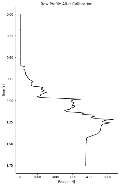
Raw Data

Below is the raw force profile. In it you can see lag time before the probe enters the snow this can make interpretation difficult. Thus we need a way to estimate where the location of the snow surface.

# Plot up the raw stuff
fig, ax = plt.subplots(figsize=(6,10))

ax.plot(df['force'], df['time'], color='k')
ax.set_title("Raw Profile After Calibration")
ax.set_xlabel('Force [mN]')
ax.set_ylabel('Time [s]')
ax.invert_yaxis()

Workflow

Assumptions:

• The two sensors are measuring the same thing above the snow

Steps:

1. Normalize the two signals using the mean value of the 1st 200 points

2. Calculate the absolute value of the active minus the ambient

3. Search for the first value greater than the threshold

n_points = 1000
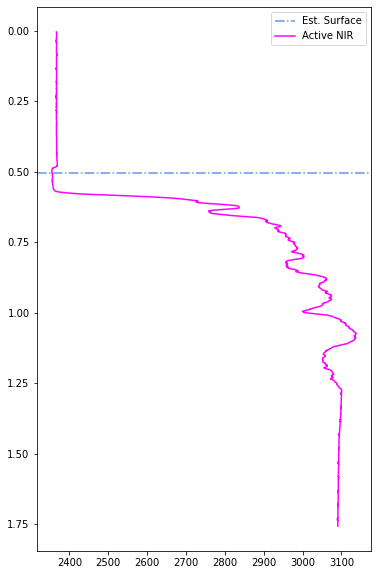
surface = get_nir_surface(df['Sensor2'], df['Sensor3'])

# Plot it up
fig, ax = plt.subplots(figsize=(6,10), ncols=1)

ax.axhline(df['time'].iloc[surface], 0, 1,linestyle='dashdot', label='Est. Surface', color='cornflowerblue')
ax.plot(df['Sensor3'], df['time'], color='magenta', label='Active NIR')
ax.legend()
ax.invert_yaxis()

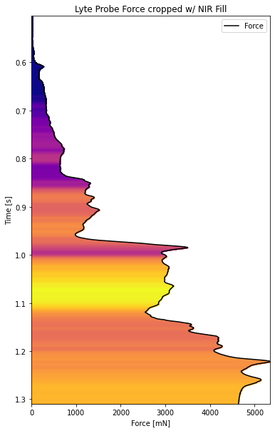
Show off a final plot!

import matplotlib
import numpy as np

cmap = matplotlib.cm.plasma
normalize = matplotlib.colors.Normalize(vmin=2900, vmax=df['Sensor3'].max())


fig, ax = plt.subplots(figsize=(6,10))
n_values = 10000

for idx in df.index[0:-1*shift]:
    d = [df['force'].iloc[idx], df['force'].iloc[idx+1]]
    indicies = [df['time'].iloc[idx], df['time'].iloc[idx+1]]
    ax.fill_betweenx(indicies, d,
                    color=cmap(normalize(df['Sensor3'].iloc[idx])))


# Plot up the force profile
ax.plot(df['force'], df['time'], color='k', label='Force')
ax.set_title("Lyte Probe Force cropped w/ NIR Fill")
ax.set_xlabel('Force [mN]')
ax.set_ylabel('Time [s]')

# Guess at bottom stop
ax.set_ylim(df['time'].iloc[surface], df['time'].iloc[21000])
ax.set_xlim(0,df['force'].max())
ax.legend()
ax.invert_yaxis()